Difference between revisions of "NeoScan Manual Part C: Near Field Mapping"
(→Scan Control Page) |
(→NeoScan Visualization Utility) |
||
| Line 510: | Line 510: | ||
During each scan, both the magnitude and the phase of a particular electric field component at a plane are measured. Measured data can easily be interpreted and understood when displayed as 2D or 3D graphs. Visualization of the [[NeoScan]] scan data are realized by LabVIEW based programs. It plots the amplitude and the phase of the measured field distribution on a horizontal plane after the scan. [[NeoScan]] Visualization Utility includes three pages: Settings, Near Field Maps, and Far Field Patterns. | During each scan, both the magnitude and the phase of a particular electric field component at a plane are measured. Measured data can easily be interpreted and understood when displayed as 2D or 3D graphs. Visualization of the [[NeoScan]] scan data are realized by LabVIEW based programs. It plots the amplitude and the phase of the measured field distribution on a horizontal plane after the scan. [[NeoScan]] Visualization Utility includes three pages: Settings, Near Field Maps, and Far Field Patterns. | ||
| − | Open the [[NeoScan]] Visualization Utility program from Desktop or Windows Explorer by double clicking on the NeoScanVisual icon. By default, [[NeoScan]] Visualization Utility program opens up with “Settings” page (Figure 5.1). | + | [[Image:icon_Plot.png|right]] Open the [[NeoScan]] Visualization Utility program from Desktop or Windows Explorer by double clicking on the NeoScanVisual icon [[Image:icon_Plot_small.png]]. By default, [[NeoScan]] Visualization Utility program opens up with “Settings” page (Figure 5.1). |
| + | |||
| + | <center>[[Image:neoscanfig_5_1.png|thumb|center|600px|<i><b>Figure 5.1</b>: NeoScan Visualizarion Utility Program.</i>]]</center> | ||
| + | |||
| + | ==== Settings Page ==== | ||
| − | |||
By default [[NeoScan]] Visualization Utility program consider the “Project Folder”: | By default [[NeoScan]] Visualization Utility program consider the “Project Folder”: | ||
C:\Users\[[NeoScan|neoscan]]\Documents\[[NeoScan]]\Projects | C:\Users\[[NeoScan|neoscan]]\Documents\[[NeoScan]]\Projects | ||
| Line 519: | Line 522: | ||
In order to view the plots of scan data: | In order to view the plots of scan data: | ||
| + | <ol> | ||
| + | <li> | ||
| + | <p> | ||
Press “Open File 1” button as shown in Figure 5.1. This opens up the dialog window, where direct you to the project in parent folder where you want to open a data file, see Figure 5.2. | Press “Open File 1” button as shown in Figure 5.1. This opens up the dialog window, where direct you to the project in parent folder where you want to open a data file, see Figure 5.2. | ||
| + | <center>[[Image:neoscanfig_5_2.png|thumb|center|600px|<i><b>Figure 5.2</b>: Selecting a data file (E_X_Dir.DAT) from project folder (patch2.349GHZ) from the dialog window.</i>]]</center> | ||
| + | </p> | ||
| + | </li> | ||
| + | <li> | ||
| + | <p> | ||
Choose the desired data file – e.g., E_X_Dir.DAT in project folder patch2.349GHz – and then press “OK” button in the dialog window. | Choose the desired data file – e.g., E_X_Dir.DAT in project folder patch2.349GHz – and then press “OK” button in the dialog window. | ||
| + | </p> | ||
| + | <ul> | ||
| + | <li> | ||
| + | <p> | ||
“Information Panel” and “Project Description” will display all scan information regarding the selected project and scan (Figure 5.3). | “Information Panel” and “Project Description” will display all scan information regarding the selected project and scan (Figure 5.3). | ||
| − | + | <center>[[Image:neoscanfig_5_3.png|thumb|center|600px|<i><b>Figure 5.3</b>: Project Description Panel and Information Panel in NeoScan Visualization Utility program.</i>]]</center> | |
| + | </p> | ||
| + | </li> | ||
| + | </ul> | ||
| + | </li> | ||
| + | <li> | ||
| + | <p> | ||
| + | Similarly, the user can open file 2, and 3 to display simultaneously. | ||
| + | </p> | ||
| + | </li> | ||
| + | <li> | ||
| + | <p> | ||
Press “Near Field Maps” tab from [[NeoScan]] Visualization Utility program to view the plots. | Press “Near Field Maps” tab from [[NeoScan]] Visualization Utility program to view the plots. | ||
| + | </p> | ||
| + | </li> | ||
| + | </ol> | ||
| + | |||
| + | ==== Near Field Maps Page ==== | ||
| − | |||
[[NeoScan]] Near Field Maps page displays either 2D or 3D plots of the amplitude and phase distribution of the scanned field from saved files. It includes 2D Plot page and 3D Plot page. | [[NeoScan]] Near Field Maps page displays either 2D or 3D plots of the amplitude and phase distribution of the scanned field from saved files. It includes 2D Plot page and 3D Plot page. | ||
| − | + | ==== 2D Plots Page ==== | |
| − | 5. | + | When you enter “2D Plot” page, 2D contour plots for amplitude and phase distributions of the scanned field are plotted and the maximum and minimum of their values are displayed in the boxes next to the graphs (Figure 5.4). |
| + | <center>[[Image:neoscanfig_5_4.png|thumb|center|600px|<i><b>Figure 5.4</b>: 2D plots in NeoScan Near Field Maps Page.</i>]]</center> | ||
| − | + | <ul> | |
| − | + | <li> | |
| + | <p> | ||
By default, the program plots fields in V/m units. You can use the key labeled “Amplitude Unit?” to display them in dBV/m (Figures 5.4 and 5.5). | By default, the program plots fields in V/m units. You can use the key labeled “Amplitude Unit?” to display them in dBV/m (Figures 5.4 and 5.5). | ||
| + | <center>[[Image:neoscanfig_5_5.png|thumb|center|600px|<i><b>Figure 5.5</b>: 2D Amplitude graphs in units of dBV/m (left) and V/m (right).</i>]]</center> | ||
| + | </p> | ||
| + | </li> | ||
| + | <li> | ||
| + | <p> | ||
The “Phase Shift” knob adds an angular shift (in degree) to the phase distribution (Figure 5.6). | The “Phase Shift” knob adds an angular shift (in degree) to the phase distribution (Figure 5.6). | ||
| + | <center>[[Image:neoscanfig_5_6.png|thumb|center|600px|<i><b>Figure 5.6</b>: Effect of 90° phase shift on 2D Phase graph.</i>]]</center> | ||
| + | </p> | ||
| + | </li> | ||
| + | <li> | ||
| + | <p> | ||
The Phase Threshold knob will sets any phase below a minimum field threshold (in V/m) to zero. Figure 5.7 compares the 2D Phase graph without a phase threshold (left) with the one with a phase threshold when the minimum field is set to 10 V/m (right). | The Phase Threshold knob will sets any phase below a minimum field threshold (in V/m) to zero. Figure 5.7 compares the 2D Phase graph without a phase threshold (left) with the one with a phase threshold when the minimum field is set to 10 V/m (right). | ||
| − | By default, [[NeoScan]] Visualization Utility program fits the 2D graphs into the square window. If the DUT is other than a circle or regular polygon such as square, equilateral triangle, etc. you must choose the “Maintain Ratio” option in “View Fit?” in order to keep the object proportional. As an illustration, Figure 5.8 presents the comparison of 2D amplitude plots for field distribution of a 12 mm × 220 mm (rectangular) slotted waveguide antenna with different view options when “View Fit?” key is set to “Fit to Window” (left plot) and when “Maintain Ratio” option is chosen (right plot). | + | <center>[[Image:neoscanfig_5_7.png|thumb|center|600px|<i><b>Figure 5.7</b>: 2D Phase graphs without (left) and with a phase threshold, setting the minimum field to 10 V/m (right).</i>]]</center> |
| + | </p> | ||
| + | </li> | ||
| + | <li> | ||
| + | <p> | ||
| + | By default, [[NeoScan]] Visualization Utility program fits the 2D graphs into the square window. If the DUT is other than a circle or regular polygon such as square, equilateral triangle, etc. you must choose the “Maintain Ratio” option in “View Fit?” in order to keep the object proportional. As an illustration, Figure 5.8 presents the comparison of 2D amplitude plots for field distribution of a 12 mm × 220 mm (rectangular) slotted waveguide antenna with different view options when “View Fit?” key is set to “Fit to Window” (left plot) and when “Maintain Ratio” option is chosen (right plot). | ||
| + | <center>[[Image:neoscanfig_5_8.png|thumb|center|600px|<i><b>Figure 5.8</b>: Comparison of 2D amplitude plots for field distribution of a slotted rectangular waveguide antenna with different view options; When “View Fit?” key is set to “Fit to Window” (left plot) and when “Maintain Ratio” option is chosen (right plot).</i>]]</center> | ||
| + | </p> | ||
| + | </li> | ||
| + | <li> | ||
| + | <p> | ||
Press “Save Graphs” button to save all plots. The plots associated with a project are saved in a folder called “Plots” within the same folder. | Press “Save Graphs” button to save all plots. The plots associated with a project are saved in a folder called “Plots” within the same folder. | ||
| − | + | </p> | |
| + | </li> | ||
| + | <li> | ||
| + | <p> | ||
You can zoom in and out the graphs by clicking on the zoom button (Figure 5.4). | You can zoom in and out the graphs by clicking on the zoom button (Figure 5.4). | ||
| − | + | </p> | |
| − | + | </li> | |
| − | + | </ul> | |
| − | + | ||
| − | + | ||
| − | + | ||
| − | + | ||
| − | + | ||
| − | + | ||
| − | + | ||
| − | + | ||
| − | + | ||
| − | + | ==== 3D Plots Page ==== | |
To view 3D plots, press the “3D Plots” tab in Near Field Maps page (Figure 5.9). | To view 3D plots, press the “3D Plots” tab in Near Field Maps page (Figure 5.9). | ||
Revision as of 20:59, 8 March 2017
Near Field Mapping
Near Field Scanning
The scanning measurement maps the electric field distribution near a device under test (DUT). During each scan, both the magnitude and the phase of the particular electric field component are measured. The probe is attached to a probe fixture mounted on the computer controlled translation stage to allow the probe to be scanned in two directions.
Requirements for Scan
The following instruments are needed for scanning measurement:
-
NeoScan Optical Mainframe
-
Either one normal or one tangential probe
-
A 2-axis translation stage
-
A RF lock-in amplifier
-
A signal generator
-
A synthesizer for generating RF source to device under test
-
A 2nd synthesizer for mixing Local Oscillator (LO) source
-
Probe fixture for translation stage
-
One GPIB-USB cable for lock-in amplifier
-
One USB multi-port Hub
-
One USB cable for optical mainframe
-
One BNC – SMA cable
-
SMA RF cables
-
BNC cables for 10 MHz reference
Scan Setup and Procedure
The setup for the scanning procedure is similar to Signal Strength Check and Probe Optimization setup as described in section 3.1.2 except for replacing the CPW with a DUT (Figure 4.1). It is assumed that NeoScan Optical Bench Manager program is running and the probes has been optimized at channels as it was discussed in section 3.3:

-
Setup the 2-axis translation stage and gently insert the probe inside the probe holder and fasten the screws (see section 2.8).
-
Set up the DUT near the reach of translation stage (and the probe on the probe fixture).
-
Plug 2-axis translation stage power cord into an electrical receptacle. Connect the translation stages as daisy chain. See section A-I.1.3 for more details.
-
Connect a USB cable from the X-axis translation stage to the USB multi-port Hub. Turn on translation stage power.
-
The probe stays connected to the correct fiber “Probe” of the NeoScan system.
-
For a tangential probe, select the E-field sensitivity direction. The probe must be oriented along the X-axis to scan the X-component of the electric field. It should be re-aligned along the Y-axis to measure the Y-component. During each scan, both the magnitude and the phase of the particular electric field component are measured.
-
Make sure the DUT is placed on a flat and level surface. Use a level for a quick measurement. Alternatively, use the micrometer mounted on top of the translation table and measure the probe height from the surface of the DUT in its three corners – as shown in Figure 4.2.
-
Open NeoScan Mapping Utility program.

NeoScan Mapping Utility Program
NeoScan Mapping Utility program is the central command center used in the 2D field scan application. The program creates the project folder, sets the appropriate parameters for lock-in amplifier, controls translation stage, including the speed setting and 2D movement settings, and scanning of an electric field. NeoScan Mapping Utility interface includes five pages:
-
Project Settings Page: Creates the project folder, sets the operating frequency and the calibration factor;
-
Hardware Settings Page: Sets the translation stage parameters including the location of the origin (scan starting point) and speed of the stage, as well as lock-in amplifier parameters;
-
Height Settings Page: Sets the Probe Height and estimates the optimal antenna scan parameters for far field pattern measurements;
-
Scan Settings Page: Sets scan parameters, including the number of scan points and the step size;
-
Scan Control Page: Scans a 2D field and display real-time near field maps.
Make sure the GPIB-USB cable from the back panel of lock-in amplifier and the USB cable from the X-axis translation stage are connected to the NeoScan USB Hub.
Project Settings Page
The NeoScan system designates C:\Users\neoscan\Documents\NeoScan\Projects as the parent folder in which all data files from a scan will be saved as project folders in this directory.
-
Create a project folder by entering the title in Project Name Entry Box and pressing “Create Folder” button.
-
Select the operation frequency from the box labeled “Frequency.”
-
Set the “Calibration Factor.”
-
“Project Description” editor enables a user to create and edit a text file.
-
The project name should have a maximum of 25 characters. Do not use “Empty Space” or any of the following characters: ` ! @ " # $ % ^ & * ( ) + = \ | / { } [ ] , > < : ; ?. Note that it is allowed to use “dot” in project name, for example, you can choose patch_2.349GHz as your project name.
-
When you start NeoScan Mapping Utility program a folder called “Untitledproject” is created automatically in parent folder. Failed to press “Create Folder” button, all data files will be written in “C:\Users\neoscan\Documents\NeoScan\Projects\Untitledproject” folder (Figure 4.4). A user can rename the files appropriately after NeoScan Mapping Utility program is stopped.
-


Hardware Settings Page
It is assumed that the users are familiar with the operation of the “Translation Stage.” Otherwise, it is highly recommended that you read Appendix A-I. Press “Hardware Settings” tab in NeoScan Mapping Utility interface (see Figure 4.5).

-
Set lock-in amplifier parameters:
-
Select the Lock-in Amplifiers for each channel using the Lock-in Amplifier Selector and set their corresponding parameters.
-
Put down the Visa menu and select the appropriate GPIB address for lock-in amplifier Visa The default is GPIB0::8::INST.
-
Set lock-in amplifier sensitivity. The sensitivity of lock-in amplifier is the rms amplitude of an input sine (at the reference frequency) which results in a full scale DC output (10Vdc).
-
Select “Time Constant” from the dropdown lists. The default for time constant of the output low-pass filter that determines the bandwidth of lock-in amplifier in 10 ms.
-
Press “Update Settings” button to reload new values when you make changes. The system will respond with "Updated settings" message in information panel to confirm the settings if the values are appropriate. Otherwise, it asks you to check the parameters.
Other parameters that should be directly set on SR844 RF lock-in amplifier – since they are not controlled (see Figure 3.13 in section 3.2.2):
- Time constant: 24 dB/oct
- Signal Input: 50 Ω Low noise
- Sensitivity: Low noise
- X display: R(dBm)
- Y display: θ
- Remote: 50 Ω external source
The signal levels at the Signal In port on the Lock-in amplifier are in the range of -100 dBm to -40 dBm or higher, depending on device one measures. It is important to set the sensitivity of the Lock-in amplifier greater than the expected input signal amplitude at the Signal Input port (from the IF Out of the optical mainframe). For example, if you expect a signal less than -67 dBm but greater than -87 dBm, set the sensitivity to -67 dBm and 100 μV (rms) setting. If the input signal is greater than the input signal setting, an OVERLOAD condition will occur and the red LED OVERLOAD indicators on the Lock-in amplifier will flash.
-
Make sure the GPIB-USB cable from the (back panel of) each lock-in amplifier is connected to the USB Hub.
-
If the largest tolerable noise signal (at the input) exceeds the full scale signal, the red LED OVLD indicators in lock-in indicate that the readings may be invalid due to an overload condition. In this situation, you many try increasing the time constant or to use a larger full scale sensitivity.
-
-
To set translation stage speed settings:
-
From “Visa COM” serial port drop-down list select the COM port that the X Linear Translation Stage is connected to. A COM port is a specific serial connection on a computer, such as COM3.
-
Set the speeds of translation stage from “Translation Speed” box (Figure 4.5). The default value is 10 mm/s – indicating that translation stage can move 10 mm per second.
-
Press “Set Speed” button to save the new settings. The system will respond with confirmation message “Set Speed OK” in information panel. The Scan Speed is ~ 0.3 mm/s.
-
When translation stages power up, they need to be homed in order to get an accurate reference position. The home sensor is at the motor end of the stage. Press “Home Position” button.
-
- In order to displace translation stage to a defined position along X-axis, enter the appropriate X coordinate in the X Position Setting Entry Box and then press “Move along X” button as shown in Figure 4.6. Similarly, enter the appropriate Y coordinate in the Y Position Setting Entry Box and then press “Move along Y” button to move to the defined position (see Appendix A-I for more details).
-
Use “Set Origin” button to define the starting point of the scanning area (Figure. 4.6). See Appendix A-I for more details.
-
To go to the origin, press “Move to Origin” button.

Height Settings Page
Set the probe height – the distance between the probe and the DUT surface – using the knob (Figure 4.7). If you are interested in high resolution scanning, you may skip the other parameters, which will be discussed later in the chapter on Far Field Measurements.

Scan Settings Page
In order to scan the distribution of electric field on a DUT, three parameters are needed to be known:
-
Dimensions of the probed (scanned) area in X and Y directions (DPX, DPY);
-
The step size ∆X and ∆Y that represents the spacing between points along X-axis and Y-axis, respectively;
-
Probe height or the distance of the probe to the DUT surface.
To be more precise, one needs Nx x Ny points to scan the whole area, where N_x=DXP/∆X and N_Y=DYP/∆Y. For instance, 4624 points (68 x 68) are needed in order to scan a 34 mm x 34 mm Patch Antenna with resolution of 0.5 mm (500 μm). The effects of the Step Size (scan resolution) and Probe Height on the 2D Amplitude near field maps for 2.349 GHz Patch Antenna are shown in Figure 4.8.

To set scan parameters, press “Scan Settings” tab in NeoScan Mapping Utility program (Figure 4.9).

-
Switch ON mode enable the user to scan the three channels simultaneously using a single Lock-in Amplifier.
-
Select the channel(s) you want to scan by checking the check boxes (Figure 4.10).
 Figure 4.10: Setting Scan Parameters in Scan Settings Tab.
-
Use the Data Label text boxes to choose a name of the files the data to be written. By default the program automatically reads the current working channel. “Information” editor enables a user to add a text on the data file header.
-
The Data Label should have a maximum of 25 characters. Do not use “Empty Space” or any of the following characters: ` ! @ " # $ % ^ & * ( ) + = \ | / { } [ ] , > < : ; ?. Note that it is allowed to use “dot” in project name.
-
-
Enter the number of points you want to scan in X and Y direction in entry boxes labeled “No. Point X” and “No. Point Y,” respectively (Figure 4.10).
-
Set the step size in each direction in entry boxes labeled “Step Size X” and “Step Size Y,” respectively. These values are in mm.
-
Select “What Axis to Scan First?” By default the program start scanning Y-axis first. In either case the scan data is written in a file in the same format, see Figure 4.11.
 Figure 4.11: Setting directions of scan using “What Axis to Scan First?” .
-
The information panel will display the total number of points that has to be scanned (Nx x Ny) in the box labeled “Total No. of Points”.
-
The program will also calculate the “Single Move Time” for each scan point (without delay) and displays the “Estimated Scan Time”.
-
The user can control the dwell time from “Dwell Control” key (Figure 4.12). The Dwell Time is the amount of time spent recording the signal for one data point for a channel before moving to the next point. By default, “Dwell Control” key is set to “Auto”. This introduces few msec dwell time during the scan. To change the dwell time, select the “Manual” option from “Dwell Control” button and enter the desired value in box labeled “Manual Move Time” in “Manual Move Setting” section (Figure 4.12). You can view the new “Estimated Scan Time” by pressing the “Update Scan Time” button.
 Figure 4.12: Manual Move Settings in Scan Settings Tab.
 -


Scan Control Page
It is assumed that the scan parameters are set and the scan measurement setup has been setup. In order to start the scan, press “Scan Control” tab in NeoScan Mapping Utility program (Figure 4.13).

-
Press “Start Scan” button to start the scan.
-
The program displays 2D Amplitude and 2D phase contour plots of the measured amplitude and phase during the scan, as shown in Figure 4.14. Graphs are rescaled continuously during the scan. This enables the users to monitor the status of the scan. For instance, any sudden change or any instrumental failure can appears as anomalous pattern in either 2D plots.
-
The “Pause Scan” and “Stop Scan” buttons control the scan process. During scanning, use “Pause Scan” to pause temporarily the scanning. Pressing the “Stop Scan” button during scanning, will stop the scanning process.
-
The “Plot Display?” key allows a user to display 2D Amplitude graph in dBm or μV unit. Similarly, “Current Signal” and “Current phase” in information panel present the lock-in amplifier current readings during the scan (Figure 4.15).
 Figure 4.14: 2D Amplitude (in dBm unit) and 2D phase contour plots of the measured amplitude and phase during the scan.
 Figure 4.15: 2D Amplitude (in μV unit) and 2D phase contour plots of the measured amplitude and phase during the scan.
-
A user can check the “Elapsed Scan Time” and view the current X and Y position of the probe from the information panel (see Figure 4.16).
-
During the scan, there is no access to other tabs or pages in NeoScan Mapping Utility program.
-
When a signal falls below -150 dBm, a warning message appear in Information Panel indicates that “Detected a signal < -150 dBm in Ch 1 -- much below the noise level.” You may check the data later.
-


The “Stop” button stops the application. To close (kill) the NeoScan window click on exit button ![]() on the top far right in the LabView user interface. To re-start running the program press the start button
on the top far right in the LabView user interface. To re-start running the program press the start button ![]() located on the top left in the LabView window, see Figures 4.5 and 4.16.
located on the top left in the LabView window, see Figures 4.5 and 4.16.

The NeoScan Scan Data
During each scan, both the magnitude and the phase of a particular electric field component at a plane are measured. When the scan is completed, data are written in .DAT files in your defined (created) project folder, say “patch_2.349GHz,” in the parent folder, i.e. C:\Users\neoscan\Documents\NeoScan\Projects\patch_2.349GHz.
For each scan the amplitude of the measured field, the phase of the field, and the scan information are written in the files – defined by Data Label – in project folder. All amplitudes are given in units of V/m and all phases in degree. The scan file also contains the basic information about the scan including the operating frequency (in GHz), correction factor, the number of points for scan and the step sizes (in mm) and etc. Figure 4.17 shows the contents of data file “E_X_Dir.DAT”, in “patch_2.349GHz” folder representing scan of 2.349 GHz patch antenna along the X direction:
During a scan, data is collected and immediately displayed by NeoScan Mapping Utility program. However, data will be written into the files at the end of the scan.

NeoScan Visualization Utility
During each scan, both the magnitude and the phase of a particular electric field component at a plane are measured. Measured data can easily be interpreted and understood when displayed as 2D or 3D graphs. Visualization of the NeoScan scan data are realized by LabVIEW based programs. It plots the amplitude and the phase of the measured field distribution on a horizontal plane after the scan. NeoScan Visualization Utility includes three pages: Settings, Near Field Maps, and Far Field Patterns.

Settings Page
By default NeoScan Visualization Utility program consider the “Project Folder”: C:\Users\neoscan\Documents\NeoScan\Projects as the parent folder in which all saved data are stored.
In order to view the plots of scan data:
-
Press “Open File 1” button as shown in Figure 5.1. This opens up the dialog window, where direct you to the project in parent folder where you want to open a data file, see Figure 5.2.
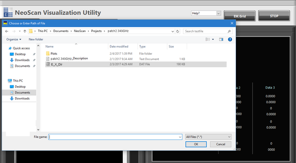 Figure 5.2: Selecting a data file (E_X_Dir.DAT) from project folder (patch2.349GHZ) from the dialog window.
 -
Choose the desired data file – e.g., E_X_Dir.DAT in project folder patch2.349GHz – and then press “OK” button in the dialog window.
-
“Information Panel” and “Project Description” will display all scan information regarding the selected project and scan (Figure 5.3).
 Figure 5.3: Project Description Panel and Information Panel in NeoScan Visualization Utility program.
-
-
Similarly, the user can open file 2, and 3 to display simultaneously.
-
Press “Near Field Maps” tab from NeoScan Visualization Utility program to view the plots.


Near Field Maps Page
NeoScan Near Field Maps page displays either 2D or 3D plots of the amplitude and phase distribution of the scanned field from saved files. It includes 2D Plot page and 3D Plot page.
2D Plots Page
When you enter “2D Plot” page, 2D contour plots for amplitude and phase distributions of the scanned field are plotted and the maximum and minimum of their values are displayed in the boxes next to the graphs (Figure 5.4).

-
By default, the program plots fields in V/m units. You can use the key labeled “Amplitude Unit?” to display them in dBV/m (Figures 5.4 and 5.5).
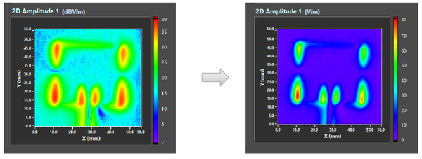 Figure 5.5: 2D Amplitude graphs in units of dBV/m (left) and V/m (right).
 -
The “Phase Shift” knob adds an angular shift (in degree) to the phase distribution (Figure 5.6).
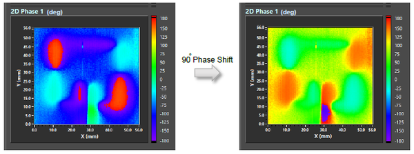 Figure 5.6: Effect of 90° phase shift on 2D Phase graph.
 -
The Phase Threshold knob will sets any phase below a minimum field threshold (in V/m) to zero. Figure 5.7 compares the 2D Phase graph without a phase threshold (left) with the one with a phase threshold when the minimum field is set to 10 V/m (right).
 Figure 5.7: 2D Phase graphs without (left) and with a phase threshold, setting the minimum field to 10 V/m (right).
 -
By default, NeoScan Visualization Utility program fits the 2D graphs into the square window. If the DUT is other than a circle or regular polygon such as square, equilateral triangle, etc. you must choose the “Maintain Ratio” option in “View Fit?” in order to keep the object proportional. As an illustration, Figure 5.8 presents the comparison of 2D amplitude plots for field distribution of a 12 mm × 220 mm (rectangular) slotted waveguide antenna with different view options when “View Fit?” key is set to “Fit to Window” (left plot) and when “Maintain Ratio” option is chosen (right plot).
 Figure 5.8: Comparison of 2D amplitude plots for field distribution of a slotted rectangular waveguide antenna with different view options; When “View Fit?” key is set to “Fit to Window” (left plot) and when “Maintain Ratio” option is chosen (right plot).
 -
Press “Save Graphs” button to save all plots. The plots associated with a project are saved in a folder called “Plots” within the same folder.
-
You can zoom in and out the graphs by clicking on the zoom button (Figure 5.4).


3D Plots Page
To view 3D plots, press the “3D Plots” tab in Near Field Maps page (Figure 5.9).
3D Amplitude graphs can be plotted either in dBV/m or V/m using the key labeled “Amplitude Unit?”
The “Phase Shift” knob adds an angular shift (in degree) to the phase distribution.
Users can choose the plot style using “Plot Style” dropdown window (Figure 5.10). It includes: cwLine cwPoint cwLinePoint cwHiddenLine cwSurface cwSurfaceLine cwSurfaceNormal cwContourLine cwSurfaceContour
The default format is “cwSurface.”
To adjust the graph degree of transparency use “Transparency” knob or Transparency Entry Box as shown in Figure 5.11.
The “Stop” button stops the application. To close (kill) the NeoScan window click on exit button on the top far right in the LabView user interface. To re-start running the program press the start button located on the top left in the LabView window, see Figure 5.1.
5.1.5 Far Field Patterns Page
The far field pattern measurement and utility are discussed in details in section 6.