Changes

The Mirage III has approximate dimensions (length,wingspan,height) of 15m x 8m x 4.5m. Or, measured in terms of freespace wavelength at 850 MHz, 42.5 lambda λ x 22.66 lambda λ x 12.75 lambdaλ. Thus, for the purposes of [[EM.Tempo]], we need to solve a region of about 12,279 cubic wavelengths. For problems of this size, a great deal of CPU memory is needed, and a high-performance, multi-core CPU is desirable to reduce simulation time.

[https://aws.amazon.com/ Amazon Web Services ] allows one to acquire high-performance compute instances on demand, and pay on a per-use basis. To be able to log into an Amazon instance via Remote Desktop Protocol, the [[EM.Cube]] license must allow terminal services (for more information, see [[http://www.emagtech.com/content/emcube-2016-licensing-purchasing-options EM.Cube]] Pricing]). For this project, we used a c4.4xlarge instance running Windows Server 2012. This instance has 30 GiB of memory, and 16 virtual CPU cores. The CPU for this instance is an Intel Xeon E5-2666 v3 (Haswell) processor.

The CAD model used for this simulation was found on [https://grabcad.com/ GrabCAD], an online repository of user-contributed CAD files and models. [[EM.Cube]]'s IGES import was then used to import the model. Once we import the model, we move the Mirage to a new PEC material group in [[EM.Tempo]].

<div><ul> <li style="display: inline-block;"> [[Image:glass.png ‎‎|thumb|left|200px|Selecting glass as cockpit material for the Mirage model.]]</li><li style="display: inline-block;"> [[Image:Mirage image.png ‎‎|thumb|left|200px|Complete model of Mirage aircraft.]]</li></ul></div>

First, we create [[Image:ff settings.png|thumb|left|150px|Adding an RCS observable with 1 degree increments in both phi and theta directions. We also create two field sensors -- one with a z-normal underneath for the aircraft, and another with an x-normal along the length of the aircraft.Mirage project]]

[[Image:ff settings===Observables===First, we create an RCS observable with one degree increments in both phi and theta directions.png|thumb|left|150px|Figure 1: Geometry of Although increasing the periodic unit cell angular resolution of the dispersive water slab in EM.Tempo.]][[Image:ff settings.png|thumb|left|150px|Figure 1: Geometry our farfield will significantly increase simulation time, The RCS of electrically large structures tend to have very narrow peaks and nulls, so the periodic unit cell of the dispersive water slab in EM.Temporesolution is required.]]

For the mesh===Planewave Source===Since we're computing a Radar Cross Section, we use the "Fast Run/Low Memory Settings" presetalso need to add a planewave source. This For this example, we will set the minimum mesh rate at 15 cells per lambdaspecify a TMz planewave with &#952; = 135 degrees, and permits grid adaptation only where necessary. This preset provides slightly less accuracy than the "High Precision Mesh Settings" preset&#966; = 0 degrees, but results in smaller meshes, and therefore shorter run times.or:

[[Image:ff settings.png|thumb|left|200px|Figure 1: Geometry of the periodic unit cell of the dispersive water slab in EM.Tempo.]][[Image:ff settings.png|thumb|left|200px|Figure 1: Geometry of the periodic unit cell of the dispersive water slab in EM.Tempo.]]<math> \hat{k} = \frac{\sqrt{2}}{2} \hat{x} - \frac{\sqrt{2}}{2} \hat{z} </math>

<br clear===Mesh Settings===For the mesh, we use the "all" Fast Run/>Low Memory Settings" preset. This will set the minimum mesh rate at 15 cells per &#955;, and permits grid adaptation only where necessary. This preset provides slightly less accuracy than the "High Precision Mesh Settings" preset, but results in smaller meshes, and therefore shorter run times.

The complete simulation, including meshing, time<div><ul> <li style="display: inline-stepping, and farfield calculation took 5 hours, 50 minutesblock;"> [[Image:Large struct article mesh settings. The average performance of png ‎‎|thumb|left|300px|Mesh settings used for the timeloop was 330 MCellsMirage project.]]</sli><li style="display: inline-block;"> [[Image:Large struct article mesh detail. The farfield computation requires a significant portion png‎|thumb|left|300px|Mesh detail near the cockpit region of the total simulation time. The farfield computation could have been reduced with larger theta and phi increments, but, typically, for electrically large structures, resolutions of 1 degree or less are requiredaircraft.]] </li></ul></div>

[[Image:Large struct article ScreenCapture3Engine settings.png|thumb|left|500px300px|Figure 1: Geometry Engine settings used for Mirage project.]]For a given system, some experimentation may be needed to determine the best number of threads to use. In many cases, using half of the periodic unit cell available hardware concurrency works well. This comes as a result of there often being two cores per memory port on many modern processors. In other words, for many problems, the dispersive water slab in EMFDTD solver cannot load and store data from CPU memory quickly enough to use all available threads or hardware concurrency.Tempo The extra threads are idling waiting for data, and a performance hit is incurred due to increased thread context switching.]]

[[Image:Large struct article ScreenCapture2.png|thumb|left|500px|Figure 1: Geometry of After the periodic unit cell of sources, observables, and mesh are set up, the dispersive water slab in EMsimulation is ready to be run.Tempo.]]  [[Image:Large struct article ScreenCapture1.png|thumb|left|500px|Figure 1: Geometry of the periodic unit cell of the dispersive water slab in EM.Tempo.]]   270 million     <br clear="all" />

[[ImageThe nearfield visualizations are also available as seen below:Large struct article RCS YZ.png‎|thumb|left|500px|Figure 1: Geometry of the periodic unit cell of the dispersive water slab in EM.Tempo.]]

<div><ul> <li style="display: inline-block;"> [[Image:Large struct article mesh detailScreenCapture1.png‎png|thumb|left|500px|Figure 1300px]]</li><li style="display: Geometry of the periodic unit cell of the dispersive water slab in EM.Tempoinline-block;"> [[Image:Large struct article ScreenCapture2.png|thumb|left|300px]]</li></ul></div>

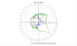
<div><ul> <li style="display: inline-block;"> [[Image:Large struct article mesh settingsRCS XY Polar.png ‎‎||thumb|left|500px300px|Figure 1XY Cut of RCS is dBsm]]</li><li style="display: Geometry of the periodic unit cell inline-block;"> [[Image:RCS ZX Polar.png||thumb|left|300px| ZX Cut of the dispersive water slab in EM.TempoRCS is dBsm]] </li><li style="display: inline-block;"> [[Image:RCS YZ Polar.png||thumb|left|300px| YZ Cut of RCS is dBsm]]</li></ul></div>